Data Engineering Certificate

What is Data Engineering ?

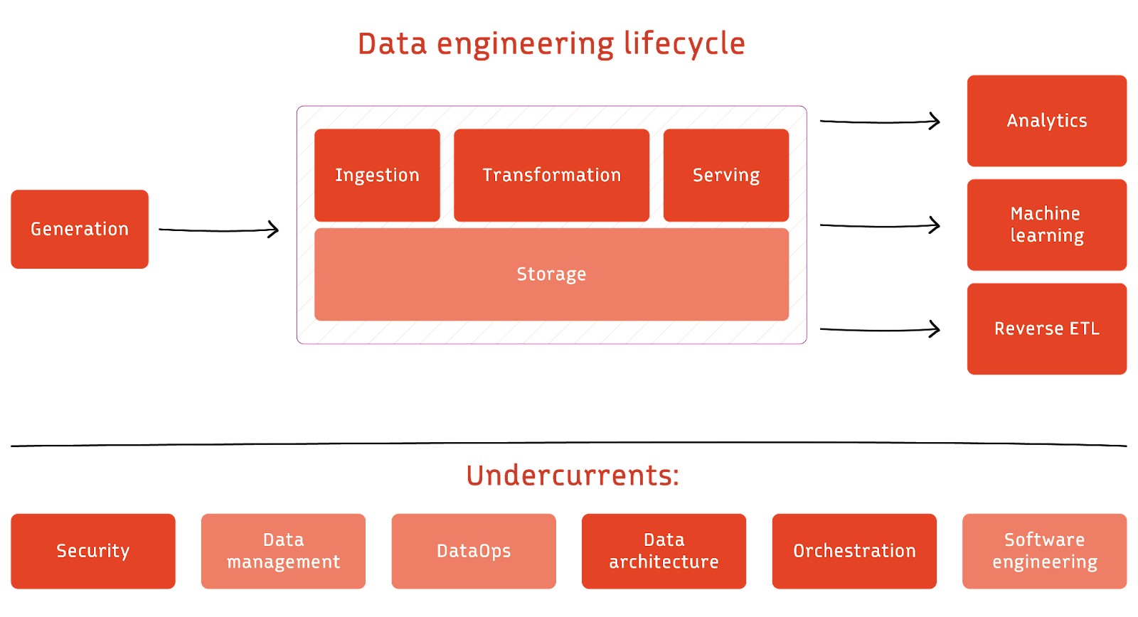
Data engineering is the development, implementation, and maintenance of systems and processes that take in raw data and produce high quality consistent information that supports downstream use cases, such as analysis and machine learning. Data engineering is the intersection of security, data management, DataOps, data architecture, orchestration, and software engineering.

-- Fundamental of Data Engineering

Data Engineering Lifecycle

Data Engineering Lifecycle -- Redpanda

Data Ingestion

Common data sources includes

• Database
• File System
• API
• File
• Data Sharing Platform
• IOT

Common challanges faced when ingesting data:

• Source system failure
• Data change
• Data schema change

Batching vs Streaming

Streaming is the process of ingesting data in real-time, where data is continuously processed once it is produced. Specific tools such as an event streaming platform or a message queue is often introduced into the pipeline to continuously ingest streams of events. Batching is essentially ingesting streaming data in large chunks, either on a predetermined time interval or size threshold.

To determine whether to use batching or streaming, consider the following:

• Costs: time, money, maintenance, and potential downtime
• Latency: Should data be processed as soon as it is produced?
• Complexity: How complex is the data pipeline? As stream processing is more complex compared to batch processing.

However, these two approaches are not mutually exclusive. In practice, a combination of both is often used to achieve the best of both worlds.

Multiple processing architectures have been proposed, such as Lambda architecture and Kappa architecture, but they were not widely adopted.

Tools such as Apache Flink now tries to unify the two approaches by treating batch processing a special case of stream processing, allowing using same code path to handle both scenarios.

Storage

• Bottom Layer: Physical storage This includes disk, SSD, and RAM.
• Middle Layer: Storage System This includes database, object/streaming storage, cache, and data storage systems such as Apache Iceberg.
• Top Layer: Storage Abstraction This includes data warehouse, data lake, data lakehouse, etc.

Queries, Modeling, and Transformations

Queries, modeling, and transformations are the processes of trnasforming data into a format that is useful for further usage.

• Queries: Issuing a request to read records from a database or other storage systems.
• Modeling: Deciding a data structure that can benefit downstearm usecases.
• Transformations: Manipulate, enhance, and save data for downstream use.

Serving

After data is transformed, it can be served to downstream use cases such as analysis(e.g BI, operational/embedded analytics), machine learning and reverse ETL.

Undercurrents of Data Engineering Lifecycle

• Security: Ensuring data is protected and accessible only to authorized parties. Defensive mindset is crucial to protect data in the cloud era.
  • Least privilege: Grant access to what is necessary is often enforced to prevent unauthorized access.
  • Data sensitivity: The best way to protect sensitive data is not to ingest it into your system in the first place.
  • In cloud scenario, understanding of topics such as IAM, encryption, and network protocol are crucial.
• Data Management: Data governance is first and foremost a data management function to ensure the quality, integrity, security, and usability of the data collected from an organization.
• Data Architecture: The design of systems to support the evolving data needs of an enterprise, achieved by flexible and reversible decisions reached through a careful evaluation of trade offs. Principles to build a good data architecture includes:
  • Choose common components wisely
  • Plan for failure: Take advantage of matrixs such as availability (SLI), reliability, and durability(Recovery Point Objective, Recovery Time Objective).
  • Architecture for scale
  • Architecture is leadership
  • Continously evolving the architecture
  • Loosely coupled architecture
  • Make reversible decisions
  • Prioritize security: Zero trust enables protection even without a perimeter.
  • Embrace FinOps: Consider cost to build sustainable systems, though it introduce challenges such as cost management.
• DataOps
  • Pillars of DataOps: Automation, Observability and monitoring, Incident response.
• Orchestration: Scheduling is prone to error and a more sophisticated approach is needed to ensure data is processed in a consistent and reliable manner; otherwise, failure in any step of the pipeline might result in a incomplete output. Common frameworks includes Airflow, Dagster, and Prefect. The dependencies between tasks are often descirbed using Directed Acyclic Graphs (DAGs).

Building a Good Data Architecture

Data architecture serves as a foundation for building a good enterprise architecture. An enterprise architecture can be defined by four parts, from top to bottom:

• Business Architecture
• Application Architecture
• Technology Architecture
• Data Architecture When designing these architectures, it is important to make decisions that are flexible and reversible, a two-way decision.

Refer to AWS Well-Architected Framework for further understanding.

Choosing the Right Tools

Common considerations when choosing tools:

• Location: on-premises, cloud, or hybrid
• Build vs Buy: Team bandwith, cost, business values
• Cost Optimization
  • Total cost of ownership (TCO)
    1. Direct cost vs indirect cost
    2. Capital expenditure (CapEx) vs operational expenditure (OpEx)
  • Total Opportunity Cost of Ownership (TOCO): The cost of being held captive to one data stack while no longer benefiting from other data stacks.
    1. Mitigate by building flexible system and identify components that are likely to change in the future.
• Team size/capabilities
• Business requirements

Thinking Like a Data Engineer

• Identify business goal and stakeholders' needs
  • Business Goal: Revenue, market share, customer satisfaction, etc.
  • Stakeholders' needs: Tools, management, system
• Define system requirements: functional vs non-functional requirements
• Choose tools and technologies
• Build, evaluate, iterate and evolve

Requirements Gathering

1. Learn what existing data systems or solutions are in place.
2. Learn what pain points or problems that are in current solution.
3. Learn what action the stakeholders plan to take based on the data.
4. Identify any other stakeholders that hold missing information.

ETL vs ELT

	ETL	ELT
Origin	Data is transformed into a predetermined format before it is loaded into a data repository. Data engineers have to carefully model the data and transform it into this format. Transformations rely on the processing power of the processing tool that is used to ingest data (unrelated to the target destination)	Raw data is loaded into the target destination then transformed just before analytics. Transformations rely on the processing power of the data repository, such as the data warehouse.
Maintenance	If the transformation is found to be inadequate, data needs to be re-loaded.	The original data is intact and already loaded and can be used when necessary for additional transformation: Less time required for data maintenance.
Load time	Typically takes longer as it uses a staging area and system. Transformation time depends on the data size, transformation complexity and the tool used.	Typically faster due to processing power and parallelization of modern data warehouse (generally considered more efficient)
Transform time	Depends on the data size, transformation complexity and the tool used.	Typically faster due to processing power and parallelization of modern data warehouse (generally considered more efficient)
Flexibility	Typically designed to handle structured data.	Can handle all types of data: structured, unstructured, semi-structured.
Cost	Depends on ETL tool used and target system the data is loaded to (And data volume).	Depends on ELT tool used and target system the data is loaded to (And data volume).
Scalability	Most cloud tools are scalable. Challenge is managing code and handling data from multiple sources when dealing with many data sources and targets.	Uses scalable processing power of the data warehouse to enable transformation on a large scale.
Data quality/security	Ensures data quality by cleaning it first. Transformations can include masking personal information.	Data needs to be transferred first to target system before transformations that enhance data quality or security are applied.

Basic Network Concepts in the Cloud

A cloud is a global network that is spread across different geographical locations known as regions. Each region contains clusters of availability zones, where each consists of one or more data centers.

Applications might spread theier resources across multiple regions and availability zones to achieve high availability, low latency, and disaster recovery.

A VPC can spread resource across multiple availability zones within a region, but cannot spread resources across regions for one VPC. For resources across different regions to communicate, configuration or mechanism such as VPC peering is required.

For VPC in the same region, resources in different VPC cannot communicate with each other as well if no additional configuration is made.

Within each availability zone, we can further divide resources into public subnets and private subnets, and each subnet can have their own ACL list to control permissions.

To access subnets, IP must be assigned to the subnet. The assigned subnet IP must be a subset of the VPC IP range.

For resources in the public subnet, each of them must have a public IP and a private IP. The public IP is used to communicate with the internet, while the private IP is used to communicate with other resources within the VPC.

It is common to have one public subnet and one private subnet in each availability zone.

Basic components in AWS that are related to network management include:

• Network Acceess Translation Gateway (NAT)

  • Allows resources in private subnets to access the internet or other resources
  • Prevents internet initating request to the private subnet.

• AWS Load Balancing (ALB)

  • Distributes traffic across multiple targets, such as EC2 instances, while ensuring the backend targets to be responsive and available while keeping the resource private to the internet.

• Internet Gateway

  • Allow network between the internet and the VPC public subnet.
  • One VPC can only have one internet gateway, and one internet gateway can only be attached to one VPC.

• Route Table

  • Essential for directing network within a VPC, where one subnet is associated with one route table.

  • A default route table (main route table) is create for the VPC on creation and allows communication between resources within the VPC, but not to the internet. Custom configuration is required to enable internet communication. For instance, private subnet can configure internet connections to the NAT located in the public subnet, and the NAT can be configured to route internet traffic to the VPC internet gateway.

  • Common basic practice is to create new route table for both public and private subnets, respectively.

  • Example

    Destination	Target
    10.0.0.6/16	Local
    0.0.0.0/0	internet-gw-id

• Security Group

  • Instance level firewall that controls the inbound and outbound traffic for EC2 instances.
  • Allows all outbound traffic and denys all inbound traffic by default.
  • A security group is associated with a VPC.
  • Stateful: Outbound traffic of an allowed inbound traffic is also allowed without needing an explicit outbound rule. This simplifies the rule management.
  • Security group chaining is a feature that allows referencingsecurity groups associated with other instances. This is useful in scenarios such as allowing an traffic fron the ALB to flow through an EC2 instance with in a private subnet.
  • It is common to only configure inbound traffic on the security group.

• Network Access Control List (ACL)

  • A layer of security at the subnet level that helps control the flow of traffic within a VPC between subnets as well as to/from the public internet.

  • Stateless: Both inbound and outbound traffic must be defined explicitly. This allows more granular control on the network security.

  • All inbound and outbound traffic are allowed by default.

  • A default rule is automatically added and cannot be removed to ensure that if a request doesn't match any of the other numbered rules, it's denied.

  • Rules are evaluated in ascending order according to the rule number until a match is found. If no match is found then the final rule (*) is applied.

  • Comparison between Security Group and Network ACL

    Security group	Network ACL
    Operates at the instance level	Operates at the subnet level
    Applies to an instance only if it is associated with the instance	Applies to all instances deployed in the associated subnet (providing an additional layer of defense if security group rules are too permissive)
    Supports allow rules only	Supports allow rules and deny rules
    Evaluates all rules before deciding whether to allow traffic	Evaluates rules in order, starting with the lowest numbered rule, when deciding whether to allow traffic
    Stateful: Return traffic is allowed, regardless of the rules	Stateless: Return traffic must be explicitly allowed by the rules

  • Example

    Rule #	Type	Protocol	Port range	Source	Allow/Deny
    100	All IPv4 traffic	All	All	0.0.0.0/0	ALLOW
    *	All IPv4 traffic	All	All	0.0.0.0/0	DENY

Based on this components, identifying the network issues can be done through a few steps:

1. Check if VPC has internet gateway
2. Check if VPC route table is properly configured.
3. Check if route table associated with the subnet is properly configured.
4. Check if security group is properly configured on services such as ALB, EC2, etc.
5. CHeck if network ACLs are properly configured.
6. Check if instances are associated with the correct security group and subnet.

DataOps

Dataops is a set of practices and cultural habits centered around building robust data systems and delivering high quality data products.

High quality data is data that is accurate, complete, discoverable, and available in a timely manner

Infrastructure as Code

Evolved from configuration management, IaC is a method of managing infrastructure through declarative codes which can be easily managed through version control and automate infrastructure state management along with CI/CD tools. Common tools includes Terraform, CloudFormation, and Ansible.

Monitoring Data Quality

Some data quality metrics examples include: ingest volumes, value distribution, null value and data freshness, etc.

Tracking all data quality metrics is impractical and might cause alert fatigue. Instead, focus on the most important metrics and set up alerts for them, meaning identify the metrics that the stackholders care about.

Using Great Expectations

Great Expectations is a tool that helps validating the input data such that the quality of the data is consistent and meets the expectations. A simple workflow consists of four steps:

1. Define Data Context: Instantiates a data context object to access the Great Expectations API.

• Great Expectations API: classes and methods to connect data sources, create expectations and validate your data

2. Define Data Source: Declare the data source, data asset and batches, the retrieve data with batch_request.

• Data source: SQL Database, a local file system, an S3 bucket, a Pandas DataFrame
• Data asset: collection of records within a data source, can be grouped in 1 or multiple batches
• Batches: partitions from your data asset
• Batch_request: primary way to retrieve data from the data asset

3. Define Expectations: Define expectations that can form an expectation suite.

• Expectation: statement to verify if data meets a certain condition such as expect_column_min_to_be_between,expect_column_values_to_be_unique, expect_column_values_to_be_null.
• Expectation suite: A collection of expectations

4. Define Checkpoints: Define checkpoints that can be used to validate the data retrieved with batch_request against the expectations defined in the expectation suite with a validator.

• Validator: Expects a batch_request and its corresponding expectation suite, then perform validation either with manual interaction or automated process using a checkpoint object
• Access metadata through backend stores: expectation store, validation store, checkpoint store, data docs.

Orchestration

Before orchestration, common tools used to set up data pipelines is cron jobs (pure scheduling). While it is simple to setup, it is not flexible and does not suitable for complex data pipelines.

With orchestration, data pipelines are often defined through a Directed Acyclic Graph (DAG), where each node represents a task and the edges represent the dependencies between tasks. Tasks can be given some criteria such as execution time, trigger type, and retry policy.

Currently, the most popular tools for orchestration is Airflow, with newer tools providing solutions to some of Airflow's shortcomings such as Dagster, and Prefect.

On AWS, alternative tools to work on orchestration includes:

• Airflow

  • Either through self-hosted Airflow or Amazon Managed Workflows for Apache Airflow (MWAA)

• AWS Glue Workflow

  • Uses Glue jobs, crwalers, triggers to form DAGs.
  • Triggers can be scheduled, on-demand, or event from services such as Amazon EventBridge.

• Amazon Step Functions

  • Orchestrate multiple AWS services and third-party applications using state machines.
  • State can be tasks that do work, such as AWS Lambda functions, EC2 task, Glue jobs, etc.
  • Input and output can be based between states.

Choosing the right tool depends on the use case and the requirements: Airflow is suitable for complex data pipelines, while Step Functions is suitable for AWS-centric workflows. Glue workflow is specifically designed for ETL processes in a serverless environment.

Airflow

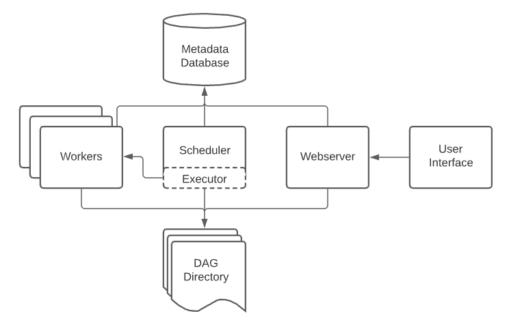
Basic components of Airflow includes:

• Scheduler: Handles both triggering scheduled workflows, and submitting Tasks to the executor to run.
• Executor: Handles running tasks. It runs everything inside the scheduler by default, but most production-suitable executors actually push task execution out to workers.
• Webserver: Presents a handy user interface to inspect, trigger and debug the behaviour of DAGs and tasks.
• DAG directory: Read by the scheduler and executor (and any workers the executor has)
• Metadata database: Used by the scheduler, executor and webserver to store state.

Airflow Components -- Airflow Documentation (Source: link)

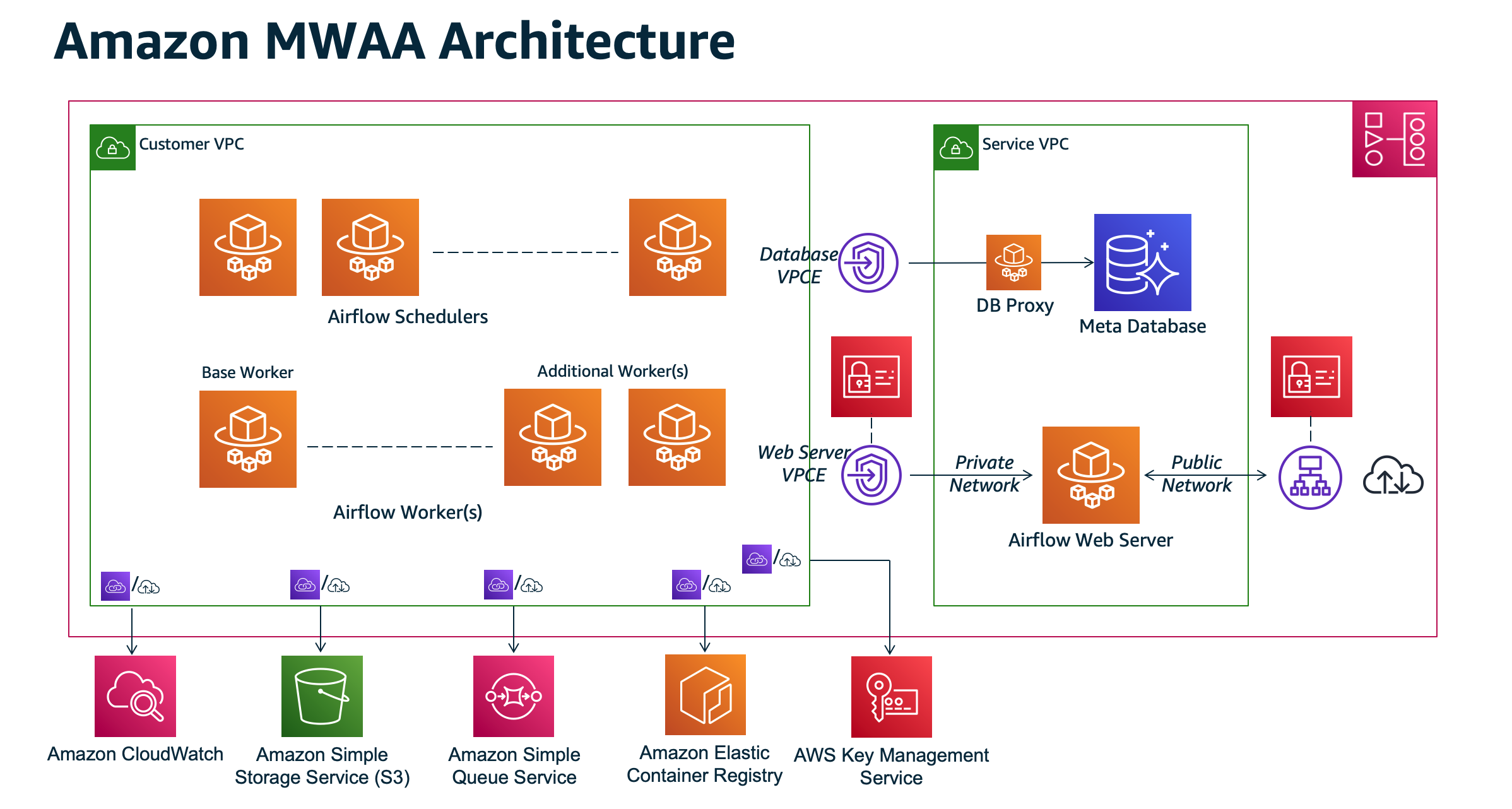
AWS provides a managed Airflow service called Amazon Managed Workflows for Apache Airflow (MWAA), which is a fully managed workflow orchestration service that enables you to create, monitor, and scale data pipelines for integrating data between AWS services and data stores.

Amazon Managed Workflows for Apache Airflow (MWAA) -- AWS Documentation (Source: link)

Usage

When working with Airflow, it should interact with storage and processing solutions using operators specifically designed for them (documentation). Airflow should only be an orchestrator, and it should delegate the actual processing workload of the pipeline to the appropriate tools such as databases or Spark clusters

Another pitfall to notice when setting the start_date parameter of a DAG is the difference between data interval and logical date. Each DAG run is associated with a data interval that represents the time range it operates in. Given a data interval, the DAG is executed at the end of the data interval, not the beginning. This is because Airflow was developed as a solution for ETL needs, where you typically need to aggregate data collected over a time interval. The logical date is a term associated with a specific DAG run, and it denotes the start of the data interval.

Airflow Operators

Airflow provides a set of operators such as EmptyOperator, PythonOperator, BashOperator, EmailOperator. Aside from those core operators provided by Airflow, there are other operators that are released independently of the Airflow core that allows you to connect to external systems. For example, operators for interacting with each AWS service, and operators used to copy data, for example, from a database to S3. It is generally recommended to use the available operators instead of writing your own code from scratch.

Airflow Dags

Dags between task are defined through bitwise operator >>. For instance,

# task_2 depends on task_1
task_1 >> task_2

# task_1 followed by two tasks, task_2 and task_3, where task_2 and task_3 is followed by task_4
task_1 >> task_2
task_1 >> task_3
task_2 >> task_4
task_3 >> task_4

With later versions of Airflow, it is recommended to use TaskFlow API to define DAGs as it is more flexible and easier to manage.

from airflow.decorators import dag, task
from datetime import datetime, timedelta

@dag(
    dag_id='taskflow_example',
    schedule_interval='@daily',
    start_date=datetime(2024, 1, 1),
    catchup=False,
    tags=['example', 'tutorial'],
    default_args={'owner': 'airflow'}
)
def taskflow_dag():

    @task(
        task_id='get_data',                    # Custom task ID
        retries=2,                             # Number of retries
        retry_delay=timedelta(minutes=5),      # Delay between retries
        multiple_outputs=True,                 # Return dictionary as multiple XCom values
        pool='default_pool',                   # Specify resource pool
        depends_on_past=False,                 # Task dependency on past runs
        execution_timeout=timedelta(hours=1)   # Max execution time
    )
    def get_data() -> dict:
        return {
            'name': 'John Doe',
            'age': 30
        }

    @task(
        task_id='process_data',
        retry_exponential_backoff=True,        # Exponential delay between retries
        max_retry_delay=timedelta(minutes=10), # Maximum retry delay
        trigger_rule='all_success'             # When to trigger this task
    )
    def process_data(data: dict) -> str:
        return f"Processed: {data['name']} is {data['age']} years old"

    # Define workflow and share data between tasks
    data = get_data()
    process_data(data)

# Create DAG instance
dag = taskflow_dag()

When defining DAGs, below parameters are crucial:

• schedule: Defines the frequency at which the DAG will be executed.
• start_date: Defines the start date of the first data interval. The start date should be static to avoid missing DAG runs and prevent confusion; static date means a fixed date like datetime.datetime(2024, 5, 20).
• catchup: Defines whether the DAG will be executed for all the data intervals between the start_date and the current date. It is recommended to set it to False to have more control over the execution of the DAG. Backfill feature can also be utilized to execute the DAG for a specific date range.

Refer to the documentation for best practices when using DAGs. Basic best practices includes:

• Keep tasks simple and atomic
• Focus on determinism and idempotence of tasks
• Avoid top-level code (in general,any code that isn’t part of the DAG or operator instantiations) as it might cause performance issues caused by the scheduler checks the DAG directory and parses the DAG files every 30 seconds. Non-top-level code is handled by the executor.
• Use variables, avoid hardcoding values.
• Organize DAGs with task groups
• Heavy loading should be offloaded to execution frameworks such as Spark.

XComs and Variables

It is common to pass data between tasks in Airflow, XComs is a simple mechanism to pass small data such as metadata between tasks by using xcom_push and xcom_pull provided through the context object. Many operators even automatically push the task results into to an XCOM key called return_value.

Note that XComs are not designed to be used for large data, it is recommended to use intermediate storage such as S3 or database to store large data then use operators to load data into downstream tasks.

from airflow import DAG
from airflow.operators.python import PythonOperator
from datetime import datetime, timedelta

default_args = {
    'owner': 'airflow',
    'start_date': datetime(2024, 1, 1),
    'retries': 1,
    'retry_delay': timedelta(minutes=5)
}

def task1_function(**context):
    # Push a value to XCom
    value_to_share = "Hello from task1!"
    context['ti'].xcom_push(key='shared_key', value=value_to_share)
    return "Task 1 completed"

def task2_function(**context):
    # Pull value from XCom
    shared_value = context['ti'].xcom_pull(key='shared_key', task_ids='task1')
    print(f"Received value from task1: {shared_value}")
    return "Task 2 completed"

with DAG('xcom_example_dag',
    default_args=default_args,
    schedule_interval='@daily',
    catchup=False
) as dag:
    task1 = PythonOperator(task_id='task1', python_callable=task1_function)
    task2 = PythonOperator(task_id='task2', python_callable=task2_function)

    # Set task dependency
    task1 >> task2

Another common way to share data across tasks is through variables. Variables is global and can avoid hard coding values inside the DAG. It is recommended to only use variables for overall configuration that covers the entire installation; to pass data from one Task/Operator to another, use XComs instead.

from airflow import DAG
from airflow.operators.python import PythonOperator
from airflow.models.variable import Variable

# Set a variable programmatically, or set through the Airflow UI
Variable.set("my_variable", "my_value")

# Get a variable
my_variable = Variable.get("my_variable")

Another useful technique to dynamically evaluate variables is through Jinja Templating.

For example, the DAG run’s logical date can be retrieved through {{ ds }} variable with a YYYY-MM-DD format. In this way, DAG run will be able to retrieve the information detailed to its execution and achieve determinism.

With Macros user can even transform or format the built-in variables. For example, the format of the {{ ds }} variable can be modified using the macros.ds_format function.

Hot, Warm, and Cold Data

These data classification is based on the data access frequency, with hot data being the most frequently accessed, followed by warm data, and cold data being the least frequently accessed.

Characteristic	Hot Storage	Warm Storage	Cold Storage
Access Frequency	Very frequent	Less frequent	Infrequent
Example	Product recommendation application	Regular reports and analyses	Archive
Storage Medium	SSD & Memory	Magnetic disks or hybrid storage systems	Low-cost magnetic disks
Storage Cost	High	Medium	Low
Retrieval Cost	Low	Medium	High

How Databases Store Data

Database often come with a software layer called DBMS (Database Management System) that handles the storage and retrieval of data.

It usually consists of four components:

1. Transport system
2. Query processor

• Query parser: Parse tokens -> check syntax & validate query -> control check -> bytecode generation
• Query optimizer: Generate execution plan based on types of operations, presence of indexes, data scan size, cost (I/O, computation, memory) and use the least expensive plan

3. Execution engine
4. Storage engine

Readings

• The Parquet Format and Performance Optimization Opportunities Boudewijn Braams (Databricks)
• Wide-column Database, Column Databases – A Deep Dive

Index

An index is a separate data structure that has its own disk space and contains information that refers back to the actual table.

On implementation level, indexes are grouped into blocks with each of them are doubly linked together to enable forward and backward reading from any block, the data stored within each block is sorted. This structure facilitates the update of the index when new data is inserted or old data is deleted.

To fully utilize the data structure, a common data structure called B-tree is built on top of the linked blocks. To locate a specific index, it is necessary to traverse the tree from the root node to the leaf node.

While traversing from the root node, it is a O(log n) operation, where n is the number of nodes in the tree. WHen reached the leaf node, it must perform a linear search to find all the data that matches the index.

Data Warehouse, Data Lake, and Data Lakehouse

Data Warehouse

Data warehouse characteristics:

• Subject-Oriented: Organizes and stores data around key business domains (models data to support decision making)
• Integrated: Combines data from different sources into a consistent format
• Nonvolatile: Data is read-only and cannot be deleted or updated
• Time-variant: Stores current and historical data (unlike OLTP systems)

Data warehouse can be implemented through different architectures:

• Big monolithic data warehouse using single server
• Data warehouse with massivly parallel processing (MPP): Scan large datasets in parallel to speed up but require conplex configuration
• Modern data warehouse: Separates compute from storage and expands the capability of MPP systems. This include Amazon Redshift, Google BigQuery and Snowflake.

A typical data-warehouse-centric architecture often works with an ETL process:

• Extract data from data sources
• Transform data at stagin area
• Load transformed data into data warehouse
• Use data marts that utilize sipmle denormalized schema to meet bussiness needs
• Perform analytic and reports based on data marts

Another model is through ELT process:

• Extract data from data sources
• Load data into data warehouse with MPP
• Transform data within data warehouse
• Data marts
• Analytic and reports

Data Lake

As data warehouse focuses on handling structured data, it is not suitable for handling unstructured data such as images, videos, and audio,. This is where data lake comes in.

A data lake is a centralized repository that ingests and stores large volumes of data in its original form. The data can then be processed and used as a basis for a variety of analytic needs.

Despite solving the problem of data warehouse, early generation data lake implementation faces other issues such as:

• Data Swamp: No proper data management, data cataloging, data discovery tools and no guarantee on the data integrity and quality
• Write-only storage such that data manipulation actions such as delete or update are hard to implement, making it difficult to comply with data regulations.
• No schema management and data modeling, making it hard to process stored data
• Data is not optimized for query operations

To address these issues, concept of data zone is introduced to the modern data lake house architecture. Data zone is used to organize data in a data lake, where each zone houses data that has been processed to varying degrees. Usally three zones are used:

• Landing/Raw zone: Houses raw data in its original format.
• Transformed/Cleaned zone: Houses data that has been cleaned and transformed for specific use cases.
• Curated/Enriched zone: Houses data that has been further processed and enriched for advanced analytics and reporting.

Data in each zone can be further partitioned based on criteria such as data, time, locattion, etc.

Data are often stored in file formats such as Parquet, Avro and Orc to optimize storage and query performance.

Another important concept is data catalog, which is a collection of metadata about the dataset (owner, source, partitions, etc.) to improve data discovery and governance.

	Data lake	Data warehouse
Type	Structured, semi-structured, unstructured	Structured
	Relational, non-relational	Relational
Schema	Schema on read	Schema on write
Format	Raw, unfiltered	Processed, vetted
Sources	Big data, IoT, social media, streaming data	Application, business, transactional data, batch reporting
Scalability	Easy to scale at a low cost	Difficult and expensive to scale
Users	Data scientists, data engineers	Data warehouse professionals, business analysts
Use cases	Machine learning, predictive analytics, real-time analytics	Core reporting, BI

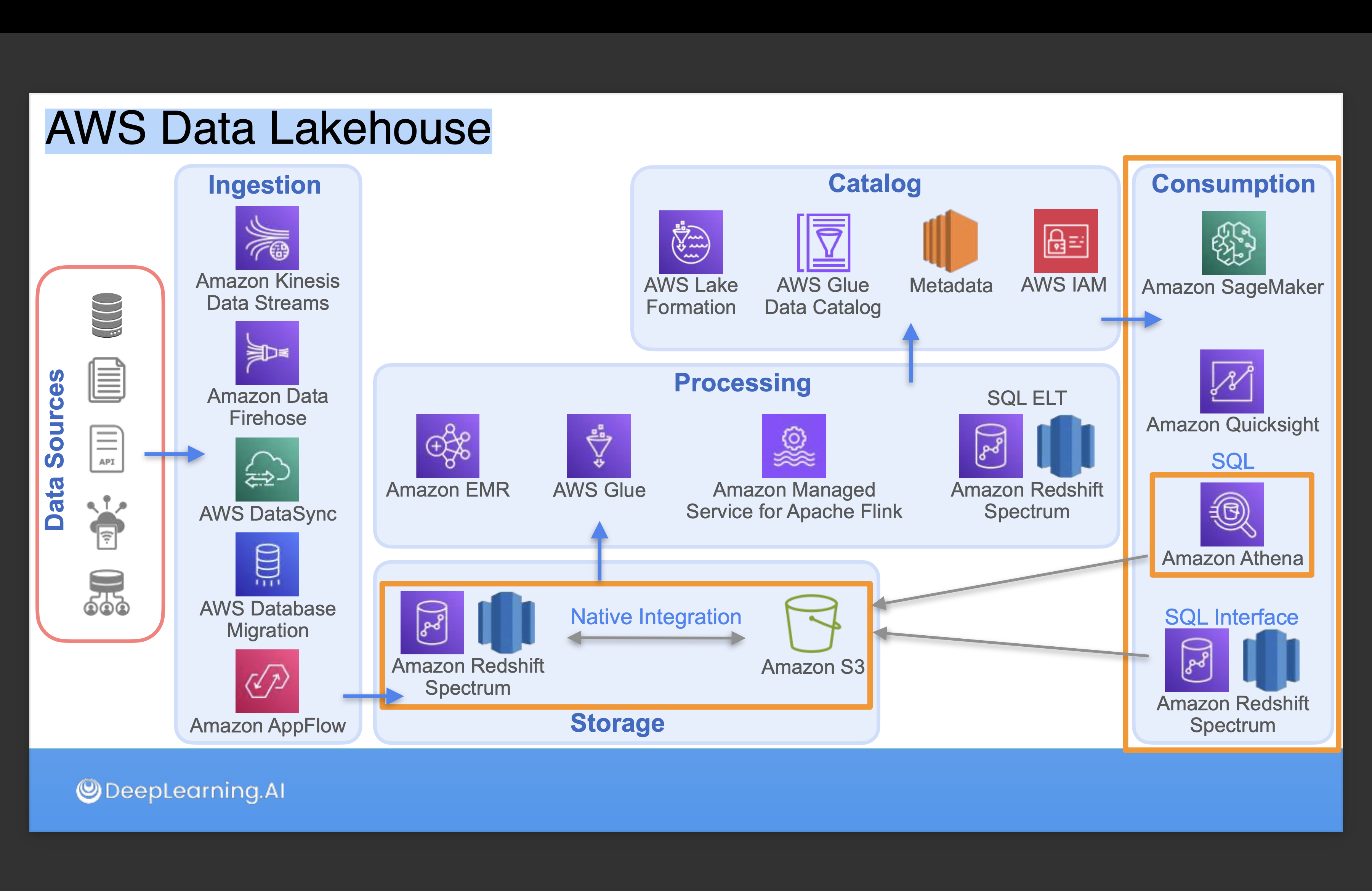
Data Lakehouse

A pipline combining both data warehouse and data lake can fully take advantage of the strengths of both architectures, but introduces higher maintenance cost. So a new architecture called data lakehouse is introduced.

At its core, a data lakehouse is very similar to a data lake. It uses a single storage layer built on top of object storage to store large amounts of data of any type. A storage layer can be organized into different zones to facilitate data governance and ensure better data quality. Databricks refers to a storage layer organized by data zones as the medallion architecture, naming the raw data zone as bronze, the clean data zone as silver, and the curated data zone containing modeled and enriched data as gold.

Furthermore, data lakehouse provides data management features (schema enforcement, schema evolution, etc), adheres to ACID principle and come with built-in data governance and security features.

To support the idea of a more transactional data lake, specialized storage formats called open table formats including Databricks Delta Lake, Apache Iceberg, and Apache Hudi are introduced.

Traditionally, setting up a data lakehouse requires a lot of steps, including: defining storage, setting up access controls, cataloging data, and managing permissions to data assets. Solutions such as AWS Lake Formation and Databricks Lakehouse Platform are introduced to simplify the process.

Example of Data Lakehouse Architecture on AWS -- Deeplearning.AI

Note that data schema evolution is a common requirement for data lakehouse, and a crawler can be used to update the schema and utilize Apache Iceberg, supported by AWS Glue data catalog, to manage the schema evolution.

Choosing the right architecture

Production Database	Data Warehouse	Data Lake	Data Lakehouse
1. Process small amounts of structured data	1. Bring together large volumes of structured / semi-structured data 2. Query current and historical data	1. Process large volumes of structured, semi-structured and unstructured data 2. Save on storage cost	1. Data management & discoverability features 2. Low latency queries
Use case: reporting, analytics	Use case: reporting, analytics	Use case: machine learning	Use case: machine learning, analytics, reporting

Data Modeling

Conceptual, Logical and Physical Data Modeling

• Conceptual data modeling:

  • Describes business entities, relationships and attributes
  • Contains business logic and rules
  • ER diagram is a common tool to represent conceptual data model

• Logical data modeling:

  • Details about the implementation of the conceptual model, including column type, pk and fk, etc.

• Physical data modeling:

  • Details about the implementation of the logical model in a specific DBMS, including data storage approach, partitioning/replication details, etc.

Normalization

The concept of normalization was first introduced by relational database pioneer Edgar Codd in 1970, and the normalization objectives that Codd outlined was:

• To free the collection of relations from undesirable insertion, update, and deletion dependencies.
• To reduce the need for restructuring the collection of relations as new types of data are introduced.

On the spectrum of normalization, there are four levels of normalization with each of them containing differnet levels of redundancy:

• Denormalized: Most straight forward form, where data is stored in a single table without any normalization that can be redundant or nested.
• First Normal Form (1NF): Each column should be unique and contain only a single value. Extra columns might be added to the table to form a composite key to serve as a primary key for the table.
• Second Normal Form (2NF): The requirements of first normal form must be met and any partial dependencies should be removed.
  • A partial dependency occurs when there is a subset of non key columns that depend on some columns in the composite key.
• Third Normal Form (3NF): All the requirements of second normal form and have no transitive dependencies.
  • A transitive dependency occurs when a non key column depends on another non key column.

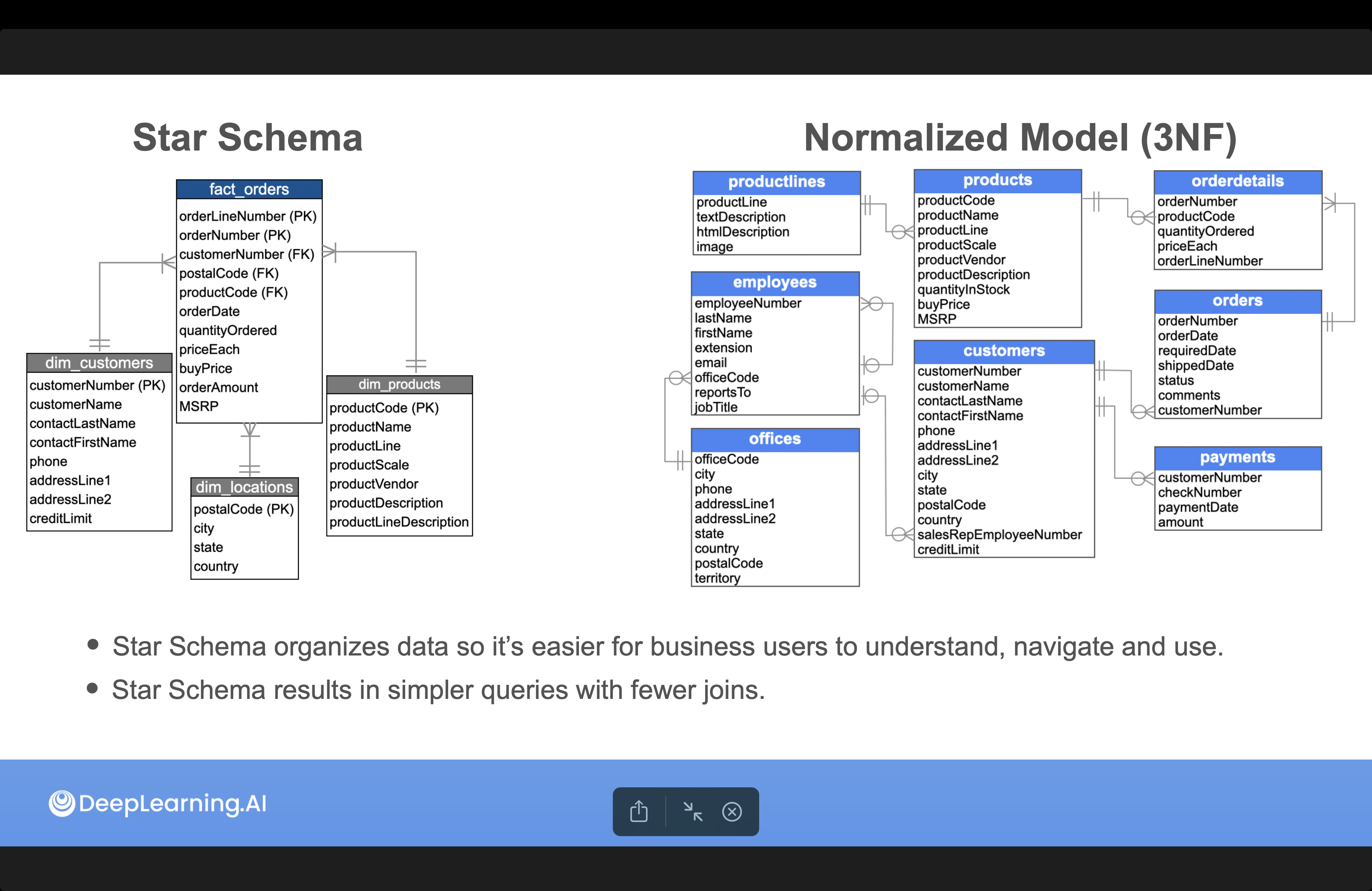
Dimenional modeling - Star schema

While normalization is a common practice in relational database, it might not be the best solution for data warehouse and analytic usages.

Complex business queries often require complex table joins and subqueires, data stored in normalized table might have issues such as higher query cost and hard to reason about.

Star schema is another approach to organize data by using fact table and dimension table:

• Fact table: Contains quantitative business measurements that result from a business event or process.
  • Each row contains the facts of a particular business event
  • Immutable (append-only)
  • Typically narrow and long
  • Has its own primary key and multiple foreign keys to refer to dimension tables
• Dimension table: Provide the reference data, attributes and relational context for the events in the fact table.
  • Describe the events’ what, who, where and when
  • Typically wide and short
  • Has its own primary key to refer to the fact table

While normalized form ensure data integrity and avoid redundancy, star schema organizes data in a way that is easier for business users to understand, as well as results in simpler queries with fewer joins.

Multiple star schema can be combined together to form a conformed dimension.

When implementing star schema, it is considered good practice to use surrogate key for the fact table.

• Used to combine data from different systems with natural primary keys that are in different formats
• Used to decouple the primary key of the star schema from source systems

Star Schema vs 3rd Normal Form -- Deeplearning.AI Data Engineering Specialization

Inmon vs Kimball Data modeling

• Inmon model:

  • Defines a data warehouse as a subject oriented, integrated, non volatile, and time variant collection of data in support of management's decisions.
  • The data warehouse contains granular corporate data that is able to be used for many different purposes, including requirements that are unknown today.
  • Source data are stored in a normalized form in data warehouse, then converted to star schema according differnt bussiness needs in the data mart.
  • Suitable when prioritizing data quality or the analysis requirements are not defined

• Kimball model:

  • Focuses more on the modeling and servers department-specific analytics directly in the data warehouse without first normalizing the data.
  • Servers department-specific analytics directly in the data warehouse using star schema without first normalizing the data.
  • Faster modeling and iteration but introduces redundancy and inconsistency.
  • Suitable when prioritizing quick insights, rapid implementation and iteration

From normalized data to star schema

1. Select the business process
2. Declare the grain
3. Identify the dimensions
4. Identify the facts

Data Vault

The Inmon and Kimball modeling approaches focus on the structure of business logic in the data warehouse. Whereas data vault focuses on separating the structural aspects of data, meaning the business entities and how they're related from the descriptive attributes of the data itself.

It uses separate tables to represent core business concepts, the relationships between those concepts, and the descriptive attributes about those business concepts. This approach only changes the structure in which data is stored:

• Allows tracing the data back to its source
• Helps avoid restructuring the data when business requirements change

The Data Vault architecture consists of three layers:

• Staging Area
  • Raw data from source systems in an insert-only manner
  • No business logic applied
  • Data is not altered in any way
• Enterprise Data Warehouse
  • Uses three types of tables: hubs, links, and satellites, to separate business objects and their relationships from their descriptive attributes
• Information Delivery Layer
  • Delivers data to the business users based on their needs using data marts, for instance, converting to star schema for analytics and reporting.

In the enterprise data warehouse, the three types of tables contains:

• Hubs
  • Contains a unique list of business keys
  • Contains hash key, calculated from the business key and used as the hub primary key
  • Contains load date, the date on which the business key was first loaded
  • Contains record source, the source of the business key
• Links
  • Connects two or more hubs
  • Contains attributes that provide context for hubs and links
• Satellite
  • • Contains attributes that provide context for hubs and links

One Big Table (OBT)

The one big table (OBT) approach is a data modeling technique that uses a single, large table that contains up to thousands of columns to store all data from all sources. Each field can contain value or nested data.

This approach avoids the need for complex joins and supports fast analytical queries.

It is becoming more popular for following reasons:

• Low cost of cloud storage
• Nested data allows for flexible schemas
• Columnar storage helps optimize the storage and processing of OBTs

However, it also has some drawbacks: store nested data:

• Business logic might be lost during analytics
• Complex data structures required to store nested data, resulting in poorer update and aggregation performance

Data Modeling and Transformation for Machine Learning

A framework for machine learning projects include multiple stages:

• Scoping: Define project
• Data
  • Define data and establish baseline
  • Determine labels required and organize data
• Algorithm Development (Modeling)
  • Prepare training datasets and test datasets
  • Select and train model
    • Classical ML algorithms: Suitable for structured data, e.g. Linear regression, Logistic regression, Decision trees, Random forest and boosted trees
    • Complex ML algorithms: Suitable for unstructured data, e.g. Deep neural networks, Convolutional neural networks, Recurrent neural networks, Recurrent neural networks, Large language models
  • Perform error analysis
  • Provide feedback to data requirements to modify input data for better model performance
• Deployment
  • Deploy in production
  • Monitor & maintain system
  • Data scientists/ML engineers will:
    • Check to make sure the system’s performance is good and reliable
    • Write software to put system into production
    • Monitor the system, track data, and maintain system
  • Data engineers will:
    • Prepare and serve the data that is needed for the deployed model
    • Serve an updated set of data to re-train and update the model

And as a data engineer, it is our job to help the organization to adopt data-centric approach to machine learning.

• Clean the data, convert it, or even create additional columns
• Shape the data into a format suitable for the ML algorithm

Feature Engineering

When performing machine learning, it is often expected to have raw data provided in a tabular format with numerical features. The process of creating new features from existing feature is called feature engineering. Given that numerical features are easier to work with and smaller feature range reduces the training time, feature engineering is a crucial step in the machine learning pipeline. Some techniques of feature engineering include:

Tabular Data

• Handling missing values
  • Methods include removing entire rows, replace with medium/mean value or similar records
  • Methods to adopt should be carefully evaluated as it may introduce bias or data loss
• Feature scaling
  • Feature values' range might affect the time needed for the model to converge as ML algorithms are essentially solving optimization problems
  • Methods include:
    • Standardization: (value - column mean)/column standard deviation, scales each feature to have mean 0 and standard deviation 1
    • Min-max scaling: (value - column min)/(column max - column min), scales each feature to a range of 0 to 1
    • One-hot encoding: Convert categorical columns into numerical ones by spreading each category into a new column with binary values, e.g. value of {red, blue, green} for color column -> divided into three columns with values {red: 1, blue: 0, green: 0}, {red: 0, blue: 1, green: 0} and {red: 0, blue: 0, green: 1}. But may introduce sparsity if the categorical column has a large number of categories.
    • Ordinal encoding: Convert categorical columns into numerical ones by mapping each category to a unique integer, e.g. value of {red, blue, green} for color column -> {1, 2, 3}.
    • Embeddings
• Converting categorical columns into numerical ones
  • Methods include one-hot encoding, label encoding and ordinal encoding
• Creating new columns by combining or modifying existing ones

Image Data

• Traditional ML approaches
  • Flatten the image into a 1D array
  • Lose spatial information that can be extracted from the relative location of pixels
  • Can create a high-dimensional vector of features, e.g. 1000 pixels by 1000 pixels → vector of size 1 million
  • Affect the performance of the ML algorithm
• Convolutional Neural Network (CNN)
  • Each layer tries to identify more image features to help with the ML task, where first layer learns generic features and later layers learn more complex patterns
  • Start with pre-trained CNN algorithms then fine tune these models for the specific task

To prepare image data for ML algorithms, data augmentation is a common technique to create new versions of existing images, such as: resizing, scaling pixels, flipping, rotation, cropping, adjust brightness, contrast, etc.

A reference code for image data preprocessing using tensoflow provided by deeplearning.ai can be checked here.

Textual Data

NLP is a subfiled of ML that focuses on working with text data. Text data often contains noises such as typos, abbreviations, and special characters, making it difficult to use directly in ML algorithms and increases training time & cost. So some preprocessing steps are often required:

• Cleaning: Removing punctuations, extra spaces, characters that add no meaning
• Normalization: Converting texts to consistent format
  • Transforming to lower-case
  • Converting numbers or symbols to characters
  • Expanding contractions
• Tokenization: Splitting each review into individual tokens (words, subwords, short sentences)
• Remove stop words: Common words that add no meaning, e.g. "the", "is", "at", "which", etc. Common libraries include nltk Gensim, TextBlob and spacy.
• Lemmatization: Replacing each word with its base form or lemma.

# Sample code for text preprocessing
import pandas as pd
import re
import unicodedata
import spacy
import numpy as np

# Sample contraction map
CONTRACTION_MAP = {
    "ain't": "is not",
    "aren't": "are not",
    "can't": "cannot",
    "cz": "because",
    "could've": "could have",
    "couldn't": "could not",
    "didn't": "did not",
    "doesn't": "does not",
    "don't": "do not",
    "gonna": "going to",
    "hadn't": "had not",
    "hasn't": "has not",
    "haven't": "have not",
    "you're": "you are",
    "you've": "you have"
}

def remove_special_char(text, special_characters = ['~','@', '#', '$', '%','^', '&', '*'], numeric = False):
    pattern = '[' + special_characters[0]
    for char in special_characters:
        pattern = pattern + '|' + char
    if (numeric):
        pattern = pattern + '|'+ '0-9'
    pattern = pattern + ']'
    return re.sub(pattern, r'', text)

def remove_accents(text):
    """
    >>> remove_special_char('déjà vu')
    'deja vu'
    """
    return unicodedata.normalize('NFKD', text).encode('ascii', 'ignore').decode('utf8')

def expand_contractions(text):
    """
    >>> remove_special_char('It couldn't be better')
    'It could not be better'
    """
    return " ".join([CONTRACTION_MAP[word] if word in CONTRACTION_MAP else word for word in text.split()])

def remove_stopwords_punctuation(text, lang_model, lemmatizing=False, stop_words=False):
    """
    >>> lang_model = spacy.load("en_core_web_sm")
    >>> remove_stopwords_punctuation('Those were amazing days!!!', lang_model, lemmatizing=False, stop_words=False)
    'Those were amazing days'
    >>> remove_stopwords_punctuation('Those were amazing days!!!', lang_model, lemmatizing=True, stop_words=False)
    'Those be amazing day'
    >>> remove_stopwords_punctuation('Those were amazing days!!!', lang_model, lemmatizing=True, stop_words=True)
    'amazing day'
    """

    doc_text = lang_model(text)
    return " ".join([token.lemma_ for token in doc_text if not(token.is_punct)]) if lemmatizing else " ".join([token.text for token in doc_text if not(token.is_punct)])

def preprocess_text(text, nlp, special_characters = ['~','@', '#', '$', '%', '^', '&', '*'], numeric = False, lemmatizing=False):
    """
    >>> lang_model = spacy.load("en_core_web_sm")
    >>> preprocess_text("\n\n\nHey that's a $$great news!!", lang_model, lemmatizing=True, stop_words=False)
    'hey that be a great news'
    >>> preprocess_text("\n\n\nHey that's a $$great news!!", lang_model, lemmatizing=True, stop_words=True)
    'hey great news'
    """

    text = remove_special_char(text, special_characters, numeric)
    text = text.lower().strip()
    text = remove_accents(text)
    text = expand_contractions(text)
    filtered_text =  remove_stopwords_punctuation(text, nlp, lemmatizing)
   
    return filtered_text

Once the text is preprocessed, it can be converted into a numerical vector using Bag of Words, TF-IDF, word embeddings and sentence embeddings.

• Bag of Words: Count the number of times each word appears in the text
  • Only takes into account the word frequency in each document
  • Some frequently appearing words might carry little meaning
• Term-Frequency Inverse- Document-Frequency (TF-IDF): Account for the weight and rarity of each word
  • TF: The number of times the term occurred in a document divided by the length of that document
  • IDF: How common or rare that word is in the entire corpus.
• Word embeddings: Convert words in to vector that captures the semantics meaning of the word
  • Libraries such as word2vec and GLOVE are trained to learn the embeddings of words from their co-occurrences.
  • Doesn't take word sequence into account, e.g. I like apple and Apple likes me will have similar embedding.
• Sentence embeddings: Convert sentences into vector that reflects the semantic meaning of the sentence
  • Results in lower dimension than the vector generated by TL-IDF
  • Open source libraries such as [SBert.net](https://sbert.net/index.html) or closed sourced models such as OpenAI, Anthropic, Gemini, etc.

# Sample code for text vectorization

# bag of words
from sklearn.feature_extraction.text import CountVectorizer

reviews = ["this wonderful price amount you get",
         "great product big amount",
         "I buy this my son his hair thin I do not know yet how well help he say smell great"]

vectorizer_bag_words = CountVectorizer(token_pattern='(?u)\\b\\w+\\b')
vectorizer_bag_words.fit(reviews)
reviews_bag_words = vectorizer_bag_words.transform(reviews)
print(vectorizer_bag_words.get_feature_names_out())
"""
['amount' 'big' 'buy' 'do' 'get' 'great' 'hair' 'he' 'help' 'his' 'how'
 'i' 'know' 'my' 'not' 'price' 'product' 'say' 'smell' 'son' 'thin' 'this'
 'well' 'wonderful' 'yet' 'you']
"""
print(reviews_bag_words.todense())
"""
[1 0 0 0 1 0 0 0 0 0 0 0 0 0 0 1 0 0 0 0 0 1 0 1 0 1]
 [1 1 0 0 0 1 0 0 0 0 0 0 0 0 0 0 1 0 0 0 0 0 0 0 0 0]
 [0 0 1 1 0 1 1 1 1 1 1 2 1 1 1 0 0 1 1 1 1 1 1 0 1 0]]
"""

# TF-IDF
from sklearn.feature_extraction.text import TfidfVectorizer

vectorizer_tfidf = TfidfVectorizer(token_pattern='(?u)\\b\\w+\\b')vectorizer_tfidf.fit(reviews)
reviews_tfidf = vectorizer_tfidf.transform(reviews)
print(vectorizer_tfidf.get_feature_names_out())
"""
['amount' 'big' 'buy' 'do' 'get' 'great' 'hair' 'he' 'help' 'his' 'how'
 'i' 'know' 'my' 'not' 'price' 'product' 'say' 'smell' 'son' 'thin' 'this'
 'well' 'wonderful' 'yet' 'you']
"""
print(reviews_tfidf.todense())
"""
[[1 0 0 0 1 0 0 0 0 0 0 0 0 0 0 1 0 0 0 0 0 1 0 1 0 1]
 [1 1 0 0 0 1 0 0 0 0 0 0 0 0 0 0 1 0 0 0 0 0 0 0 0 0]
 [0 0 1 1 0 1 1 1 1 1 1 2 1 1 1 0 0 1 1 1 1 1 1 0 1 0]]
"""

Readings

• All you need to know about encoding techniques
• From Word Embeddings to Sentence Embeddings -- Part 1
• Glossary of Deep Learning: Word Embedding
• Cohere Embeddings Docs
• Best Embedding Model -- OpenAI, Cohere, Google, E5-BGE

Data Transformation

The transformation stage of the data engineering life cycle is where data is manipulated and enhanced for downstream stakeholders.

In a data warehouse architecture, data can leverage massive parallel processing for data modeling using modeling techniques such as star schema or data vault for analytics and reporting.

In a data lake architecture, data can be transformed by applying a series of transformations by moving data from the raw to the cleaned/transformed zone. Finally, to the enriched zone so that it's ready to be consumed by data users.

During the transformation stage, some technical considerations must be considered:

• Batch transformation
  • Data size
  • Hardware specification
  • Performance specification
  • Tools such asHadoop (disk-based storage and processing) vs Spark (memory-based processing)
• Streaming transformation
  • Latency requirements
  • Micro-batching vs streaming
  • Tools such as Apache Flink + Apache Kafka
• Transformation approach
  • Single machine or distributed
  • SQL or Python

Batch Transformation

• ETL: Eatract from source data -> Transform in staging area -> Load into data warehouse
• ELT: Eatract from source data -> Load into data warehouse -> Perform transformations in data warehouse
• EtTL: Eatract from source data -> Simple transformations (clean missing values, deduplication, etc) -> Load into data warehouse -> Further transformations

During the transformation phase, taking messy/malformed data and turn it into clean data is often referred to as data wrangling. While wrangling data with self-built tools is possible, it is often more efficient to use existing libraries and tools, such as : AWS Glue DataBrew.

Another common need is to transform data for data updating. Approaches include:

• Truncate and reload: Delete all existing data and reload the entire dataset, only suitable for small dataset or data that aren't updated frequently.
• CDC: Only identify the changes in the data, then apply the changes to the data warehouse.
  • For updates, can be done with insert-only (mark old data as deleted) or upsert (insert and update).
  • For deletes, can be done with hard delete (to comply with data regulations, performance considerations, etc) or soft delete (mark data as deleted).

While single-row insertions are common in row-oriented databases, it may cause performance issues if applied to OLAP column-oriented databases. Batch insertions are more efficient in this scenario.

Distributed Processing Framework

• Hadoop

  • Uses HDFS to break large files into smaller blocks (few hundred megabytes each) and stored across multiple nodes.
  • Compute and storage is executed on the same node, whereas object storage (e.g. Amazon S3) typically has limited compute resources.
  • A name node maintains metadata such as directories, file metadata, and block locations catalog that can be used to configure data block distribution to provide redundancy (typically 3 copies) and high availability.
  • Utilizes MapReduce model for parallel processing. Steps include:
    • Map: Generate key-value pairs based on the processed data
    • Shuffle: Redistribute the data accross nodes based on keys
    • Reduce: Aggregate the data by key
  • Uses short-lived MapReduce tasks that simplifies tate and workflow management, as well as minimize memory consumptions.
  • Reads data from disk and writes intermediate computations to disk, causing high disk bandwidth utilization and increases processing time

• Spark

  • A computing engine designed for large dataset processing that addresses some shortcomings of Hadoop by supporting in-memory storage for intermediate results and interactive processing of the data.
  • A unified platform that supports analytical workloads such as SQL queries, streaming, machine learning and graph processing.
  • Cluster manager allocates resources to driver node (central controller) and worker node (executors)
  • Driver node starts a Spark session and converts user code into spark jobs that are exectued one by one based on priority. Each job can be furhter break down into multiple stages with stage dependencies defined with a DAG.
  • Each stage can be break down into multiple tasks that can be executed in parallel, and are distributed across executors to process in parallel. Results are returned to the driver node and aggregated to produce the final result.
  • Spark dataframes (high-level API) are based on Resilient Distributed Datasets (RDD, low-level API), which represents the actual partitioned collection of records that can be processed in parallel. Both are immutable data structures that guarantee the resilience of the data.
  • Operations on dataframes can be classified into transformation and action.
    • Transformation: Executed lazily (does not mutate the original dataframe and recorded as a lineage of operations) and only executed when an action is called. This includes filtering, selecting, joining, goupring, etc.
    • Action: Triggers the execution of the transformation and. This includes count, show, save, etc.
  • Immutability enables fault-tolerance of dataframes and lazy evaluation optimizes the execution plan.

Streaming Transformation

Streaming transformation prepares data for downstream consumption by converting a stream of events into another stream with enriched data, joining the stream with other streams, or performing windowed queries, etc.

• Spark streaming processes stream data in a microbatch stream processing manner, with each batch processed parallelly.
• Flink processes stream data in a true stream processing manner, with each event processed in real-time one at a time. Each node listens to messages and updates its dependant nodes, allowing delivery of processed event at low latency but come with high overhead.

When choosing a streaming engine, consider the following:

• Usecase
• Latency requirements
• Performance capabilities of the stream processing framework

Serving Data for Analytics and Machine Learning

References

• Data Engineering 101 -- Redpanda
• AWS Well-Architected Framework
• AWS Well-Architected Labs
• Questioning the Lambda Architecture -- Jay Kreps
• A Brief Introduction to Two Data Processing Architectures: Lambda and Kappa for Big Data -- Towards Data Science
• What is an AWS S3 Delete Marker?
• Airflow Documentation
• Airflow Best Practices
• A Deep Dive into Parquet: The Data Format Engineers Need to Know

---